GAMM analysis – can complexity tell us anything we don’t already know?

Sleep, heart-rate variability (HRV), and the hope of a clear link between them have kept us busy for three blogs now. In the first two, we mapped the data landscape, and in the third, we demonstrated that day-to-day sleep duration has a minimal effect on next-morning HRV. This time we reach for a more flexible statistical lens: the generalised additive mixed model, or GAMM. Think of a GAMM as a statistical Swiss‑army knife able to handle wiggly, non‑linear trends and patchy human data ,  all while respecting the fact that repeated nights from the same person are not independent. Below, I try to explain why this approach is a good fit for sleep science, walk through the model, and examine what 1,199 adults revealed when their nightly records were processed through this pipeline.

Methodology

Why GAMM and not a straight line?

Classic linear models assume that the relationship between X and Y is straight and that all observations are independent. Our experience with biology suggests otherwise. HRV often exhibits plateau effects, rebounds, and oddly timed dips; sleep duration fluctuates with weekday routines, seasons, and mood. In reality, we shouldn’t expect biological relationships to be linear in the first instance! Especially as we are looking for correlations here and not causal relationships. If we take a moment to think about sleep, it seems intuitive that both low and high levels of sleep are linked with bad general health in the next few days, while medium sleep times are probably good. This would show up on a chart as an inverted U shape.

A generalised additive mixed model (GAMM) replaces each straight line with a smooth curve built from many tiny splines, letting the data choose the shape rather than forcing it. The mixed part incorporates random effects, acknowledging that Alice’s baseline HRV differs from Bob’s, and that one person's experience on Tuesday is not the same as another’s. In practice, a GAMM can simultaneously model a wiggly group‑level curve while giving every participant their own intercept and, if needed, their own random slopes.

Dataset at a glance

Characteristic	Value
Nights analysed	89 628
Participants	1 199
Metric pairing	Sleep(t) → ΔHRV(t + 1) ( HRV(t + 1) − HRV(t))
Z‑score distributions	Sleep μ ≈ 0, σ ≈ 1.002; ΔHRV μ ≈ 0, σ ≈ 1.003
Extreme deviations (Z < –1.5)	Sleep 6.9 %; ΔHRV 6.6 %; both together 0.5 %

Table 1: Key characteristics of the sleep and HRV dataset.

We again used rolling 28‑day Z‑scores to centre each participant on their own baseline and to render nightly values comparable. Sleep slopes over 3, 5 and 7 days were appended to test whether trends, rather than single nights, carried more predictive weight.

Headline Findings from the GAMM Analysis

The Overall Population Curve

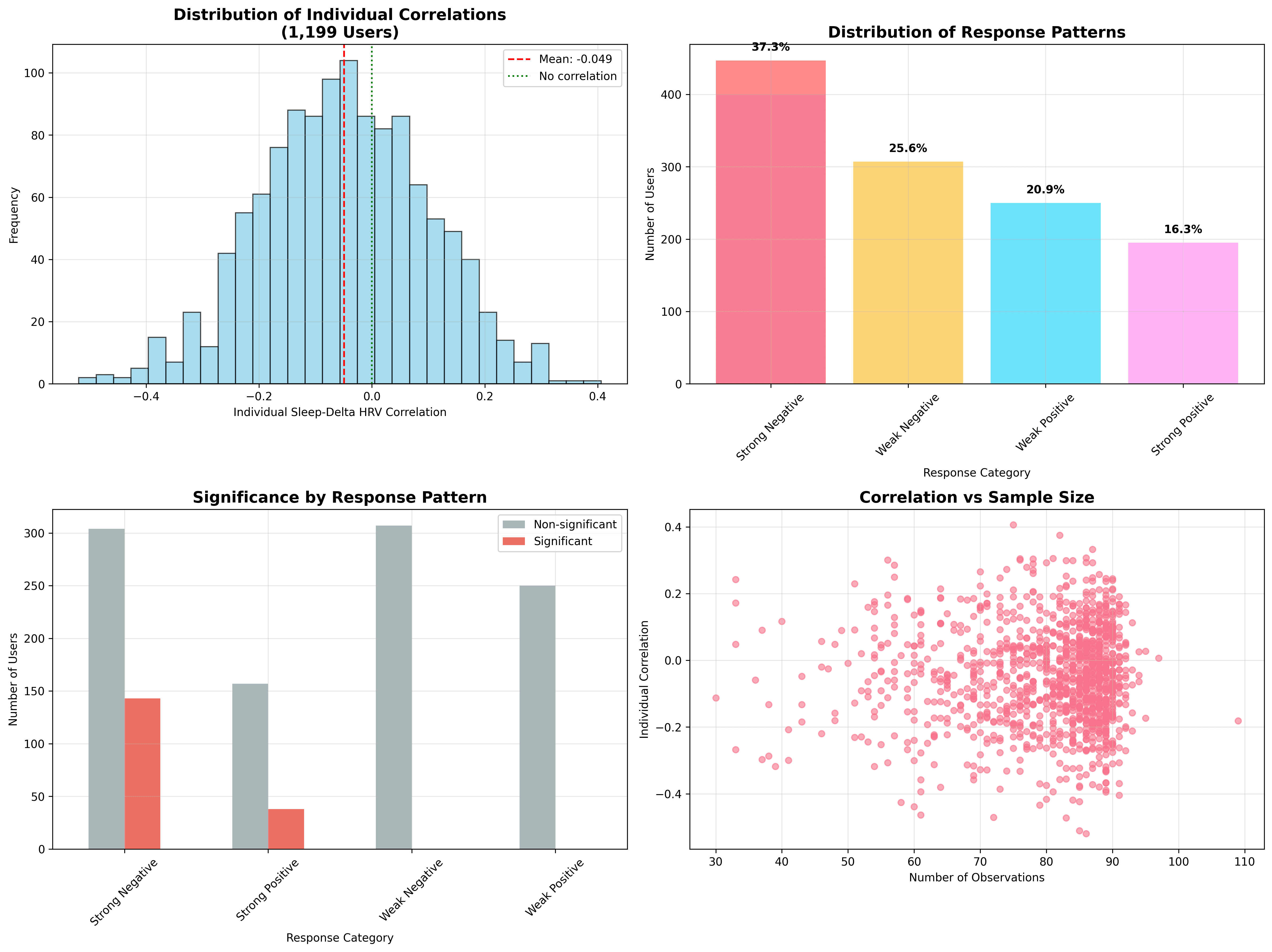
The link between sleep duration and ΔHRV is, well, almost flat. The model reports an average correlation of r = –0.0431 (p < 0.001). As we saw in the previous results, there is a statistically significant effect due to sample size, but it is a very small one. Longer‑than‑usual sleep is, if anything, associated with slightly more minor HRV upticks — the mirror image of what many self‑trackers expect.

Figure 1: The wild spread of correlations; only 15% of users (dark shading) reach within-person significance.

Within‑person versus between‑person

A GAMM lets us decompose change into two directions. Within‑person describes how deviations from an individual’s own average sleep relate to their own HRV the next day; between‑person compares long‑sleepers to short‑sleepers. Within‑person, we saw r = –0.0508 (p < 0.001) — about the same negative slope but fractionally stronger than the overall. Between‑person the relationship all but vanishes: r = –0.0065 (p = 0.045). Translation: whether you are a six‑hour sleeper or an eight‑hour sleeper, on average, has almost no bearing on how your HRV changes, but if you sleep more than your usual amount tonight, you may see a slightly dampened HRV change tomorrow. This highlights what we already know: HRV is a highly individual metric.

Individual fingerprints

Digging into the random‑effect estimates reveals that the cohort is a patchwork. The mean within‑user correlation is –0.0493, but values span from –0.52 to +0.41. 37 % of participants display positive correlations. In simple terms, some people experience the “expected” pattern (more sleep, bigger HRV uptick), some show the opposite, and many show nothing at all. Only 15% of people reach within-user statistical significance, despite vast amounts of data.

Model fit and seasonal ripples

Even with all that wiggle room, the GAMM explains a modest slice of variance: R² = 0.0019 for the linear base, nudging to 0.0023 with a shallow polynomial. Put differently, sleep duration in isolation accounts for less than a quarter of one per cent of the night‑to‑night HRV story.

A gentle sinusoid runs through the calendar: March sees a fractional uptick (+0.17 ms), April and May dip, June bounces back. Light exposure, pollen, holiday rhythms? The model cannot say, only that HRV change is not season‑proof.

Discussion

Why the counter‑intuitive sign?

We again find that more sleep tends to precede smaller HRV gains or even losses. We have several hypotheses for this:

Compensation — after a short night, our nervous system may stage a parasympathetic rebound, lifting HRV.
Reverse causality — people who feel under the weather (low HRV) may extend sleep, but the underlying stressor still drags HRV down, making the correlation appear negative.
Measurement horizon — a 24‑hour lag might miss delayed recovery curves that play out over longer horizons.
Confounding behaviour — heavy exercise days (or other HRV-suppressing factors) could be triggering extra sleep, and transiently suppressing HRV.
Noisy data - We can’t discard the fact that the raw data is still noisy, and our data processing (Outlier removal) still isn’t up to scratch.

The Power of Variability: Why "Wobbly" Sleepers Show Stronger Links

Before diving into predictive modelling, I audited which baseline characteristics distinguish the spectrum of responses. The analysis split individual correlations into four bands (strong negative, weak negative, weak positive, strong positive) and examined 24 candidate moderators.

High variability dominates. Users with greater weekday sleep variance (r = 0.166), wider sleep range (r = 0.161) and higher sleep SD (r = 0.155) tended to show stronger absolute correlations, whether positive or negative.
Shape matters. Skewness in sleep (r = 0.131) and in ΔHRV (r = –0.088) suggests that asymmetric distributions may be a driver of reactivity.
HRV volatility contributes. HRV coefficient of variation (r = –0.087) and mean HRV (r = 0.053) added smaller but still notable explanatory power.

In short, variable sleepers — the people whose bedtimes and durations bounce around — are the ones whose HRV is most likely to dance in response. Consistent sleepers tend to follow a flatter physiological track.

A side analysis grouped users by correlation sign and magnitude. Strong‑negative responders (37 %) clocked markedly higher night‑to‑night sleep variability: weekday variance r = 0.166, sleep range r = 0.161, SD r = 0.155. Skewness and kurtosis of sleep distribution also mattered. In essence, the shape of someone’s sleep pattern predicts how tightly their HRV shadows it. Consistent sleepers rarely show dramatic coupling, whereas roller‑coaster sleepers can be either strongly positive or strongly negative responders. This could be a demonstration of circulator logic going on here; the more stable (in general) the nervous system, the better the sleep and so on.

Permutation safety net

To guard against patterns born of chance, I permuted each person’s sleep series 1,000 times, recalculated correlations and applied a Benjamini–Hochberg false‑discovery gate. Only 33 users (2.8 %) survived as bona fide responders. Their shared hallmark? Elevated sleep variability and slightly higher data density (86 versus 83 observations). Average sleep length and mean HRV were indistinguishable from the crowd. Even among this select group, effect sizes hovered in the “small” aisle, underscoring that truly robust sleep–HRV links are collectable but uncommon.

Digging deeper: Predictive modelling

Can We Predict Who Will Respond?

Correlations and smooth curves tell us what happened, but can we anticipate for whom these patterns matter? To answer that, I trained an ensemble of models, with a random forest emerging as the pragmatic winner for transparency and modest overfit control. The target was each individual’s within‑user correlation strength. Predictor candidates covered 24 baseline descriptors: measures of central tendency (means, medians), spread (standard deviations, ranges, coefficients of variation) and shape (skewness, kurtosis) for both sleep and ΔHRV, plus weekday variance, seasonality metrics and simple demographics.

The resulting forest explained 5.4 % of the variance in correlation strength (R² on a three‑fold cross‑validation) and, when recast as a classifier splitting the top quartile (“strong responders”) from the rest, achieved an F1 of 0.103. In practical terms, if you took the model’s “high-responder” list of 100 users, perhaps 15–20 would actually prove to have strong sleep-HRV coupling, and you’d still miss the majority of true responders lurking in the remaining 1,099 users. An F1 score of 0.103 indicates that the current random-forest classifier offers only modest improvement over chance in identifying individuals whose HRV strongly mirrors their sleep variability. It serves as a starting point, not a clinical decision tool.

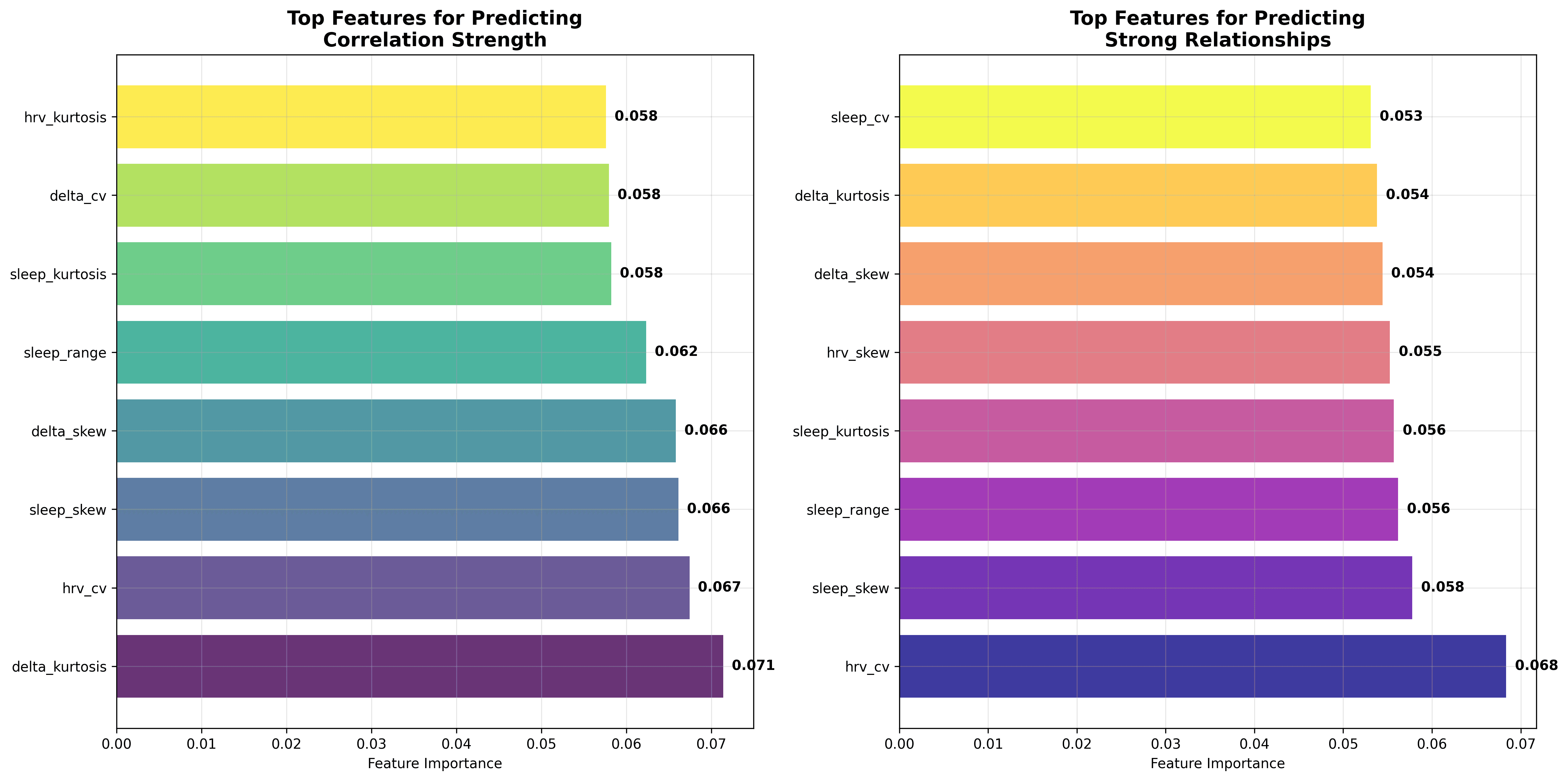
The unsurprising hero was distributed shape. Delta‑HRV kurtosis, HRV coefficient of variation and sleep skewness together explained more signal than all mean levels combined. In plainer language, how much your nightly stats zig‑zag and how lopsided those zig‑zags are tells us more about sleep‑HRV coupling than whether you usually clock seven or eight hours.

Figure 2: Top Predictive Factors: Distribution shape factors (kurtosis, skew) are most important for prediction., Strong relationship predictors include: Sleep CV, delta kurtosis, HRV CV, sleep range, and mean sleep

Identifying responder profiles

I projected predicted scores into four pragmatic buckets:

Very high responders (≈9 % of users): highly variable HRV and sleep, peaky HRV‑change distributions, skew towards either very short or very long nights.
High responders (15 %): still variable but less extreme, sometimes propelled by weekday–weekend swings.
Medium responders (43 %): the statistical bulk — mild variance, symmetrical distributions, tepid correlations.
Low/non‑responders (33 %): sleepers whose HRV barely registers bedtime tweaks.

Conclusion

Practical implications

Personal rather than populational. Whether extra sleep boosts or blunts your HRV is an individual trait. Track your own trend for a few months before concluding. If you are building scores for populations, think about making them indivdual.
Consistency still wins. Stable sleepers experience flatter HRV swings, which many athletes consider a sign of robustness.
Single‑metric coaching is risky. Basing recovery advice solely on sleep hours overlooks factors such as stress, training load, illness, and circadian cues, all of which are reflected in HRV.
High‑variability users merit attention. Their nervous systems appear more reactive to bedtime changes, making them prime candidates for personalised interventions.
Prediction helps triage. Even a modest model can flag the users most likely to benefit from tailored guidance, boosting efficiency for coaches and clinicians.

Limitations and future study

Our GAMM uses nightly duration, not sleep architecture. It assumes a 24‑hour lag captures some causality, overlooks naps, and inherits the noise of photoplethysmographic HRV. Chronotype, caffeine, menstrual phase, ambient temperature and many other factors sit outside the model but are clearly present in our physiology. Lastly, while splines capture smooth curves, they can obscure rapid step changes; complementary approaches, such as change-point detection, might sharpen insight. We will be including other factors over the next few weeks.

I still can’t discount the fact that noise is obscuring underlying links in the data. We are currently working hard on a data cleaning and standardisation pathway that we will be implementing in research.

I do think we’ve shown that prediction modelling shows we can identify those reactive sleepers with fair accuracy, paving the way for more innovative and individualised interventions.